I like playing with equations, particularly those dealing with chaos.
There is a simple recurrence relation called the logistic map that is usually pointed to as the archtypal example of chaotic behaviour emerging from a simple non-linear equation.
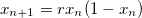
I wrote a small program to iterate the above formula for different values of r and starting values of x, and I was able to reproduce the bifurication diagram that illustrates the emergence of chaotic behaviour as r increases.
I then tried different recurrence relations to see if I could find any other interesting chaotic behaviour, and I found one that appears to display similar behaviour as the logistic map
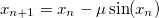
It produced a symmetrical version of the logistic map, centred on zero:

The two recurrence relations appear to be quite different, but they seem to produce similar chaotic behaviour. This recurrence formula is actually based on Kepler’s equation, and in fact it is possible to solve Kepler’s equation using fixed point iteration after a simple re-arrangement of the equation. Though the figure above does not display solutions to Kepler’s equation, if it did then there would be a major discrepancy between theory and observations.
If you find this interesting, try playing with the code and experiment for yourself. And if you come across an other interesting relations, feel free to share, I’d be curious to know.